Bulk RNA-seq Deconvolution with CIBERSORTx

workflowr

• Summary
• Checks
• Past versions

Last updated: 2026-04-14

Checks: 7 0

Knit directory: dge-analysis/

This reproducible R Markdown analysis was created with workflowr (version 1.7.1). The Checks tab describes the reproducibility checks that were applied when the results were created. The Past versions tab lists the development history.

---

R Markdown file: up-to-date

Great! Since the R Markdown file has been committed to the Git repository, you know the exact version of the code that produced these results.

Environment: empty

Great job! The global environment was empty. Objects defined in the global environment can affect the analysis in your R Markdown file in unknown ways. For reproduciblity it’s best to always run the code in an empty environment.

Seed: set.seed(20230618)

The command set.seed(20230618) was run prior to running the code in the R Markdown file. Setting a seed ensures that any results that rely on randomness, e.g. subsampling or permutations, are reproducible.

Session information: recorded

Great job! Recording the operating system, R version, and package versions is critical for reproducibility.

Cache: none

Nice! There were no cached chunks for this analysis, so you can be confident that you successfully produced the results during this run.

File paths: relative

Great job! Using relative paths to the files within your workflowr project makes it easier to run your code on other machines.

Repository version: 237c9eb

Great! You are using Git for version control. Tracking code development and connecting the code version to the results is critical for reproducibility.

The results in this page were generated with repository version 237c9eb. See the Past versions tab to see a history of the changes made to the R Markdown and HTML files.

Note that you need to be careful to ensure that all relevant files for the analysis have been committed to Git prior to generating the results (you can use wflow_publish or wflow_git_commit). workflowr only checks the R Markdown file, but you know if there are other scripts or data files that it depends on. Below is the status of the Git repository when the results were generated:

Ignored files:
    Ignored:    .DS_Store
    Ignored:    .github/.DS_Store
    Ignored:    dge-analysis/.DS_Store
    Ignored:    dge-analysis/.Rhistory
    Ignored:    dge-analysis/.Rproj.user/
    Ignored:    dge-analysis/.cursor/
    Ignored:    dge-analysis/AGENTS.md
    Ignored:    dge-analysis/analysis/.DS_Store
    Ignored:    dge-analysis/data/.DS_Store
    Ignored:    dge-analysis/output/.DS_Store
    Ignored:    dge-analysis/output/all-samples-analysis/
    Ignored:    dge-analysis/output/deconvolution/
    Ignored:    dge-analysis/output/publication-analysis/publication-analysis.RData
    Ignored:    dge-analysis/output/subgroup-chrn-analysis/CHRN-subgroup-analysis.RData
    Ignored:    dge-analysis/output/subgroup-hpp-analysis/HPP-subgroup-analysis.RData
    Ignored:    dge-analysis/output/subgroup-ion_channel-analysis/Ion_Channel-subgroup-analysis.RData
    Ignored:    dge-analysis/output/subgroup-mito-analysis/Mito-subgroup-analysis.RData
    Ignored:    dge-analysis/output/subgroup-potassium-analysis/
    Ignored:    dge-analysis/output/subgroup-rbc-analysis/RBC-subgroup-analysis.RData
    Ignored:    dge-analysis/renv/.DS_Store
    Ignored:    dge-analysis/renv/library/
    Ignored:    dge-analysis/renv/staging/
    Ignored:    phenotypic-analysis/.DS_Store
    Ignored:    variant-findings-plot/.DS_Store

Untracked files:
    Untracked:  dge-analysis/data/CIBERSORTx_Job1_output/
    Untracked:  dge-analysis/data/CIBERSORTx_Job2_output/
    Untracked:  dge-analysis/data/id_map.csv
    Untracked:  dge-analysis/output/publication-analysis/degs_padj_0.1.png
    Untracked:  dge-analysis/output/publication-analysis/supplemental_figure_4_significant_degs_padj_.05.png

Unstaged changes:
    Modified:   dge-analysis/analysis/_site.yml
    Modified:   dge-analysis/analysis/custom.css
    Modified:   dge-analysis/analysis/head.html
    Modified:   dge-analysis/code/helpers.R
    Modified:   dge-analysis/output/publication-analysis/Supplemental Table 5. Significant Differentially Expressed Genes.csv
    Modified:   dge-analysis/output/publication-analysis/batch-correction-limma/plot-counts/genes-of-interest/ACACB-subsetted-plot-counts.png
    Modified:   dge-analysis/output/publication-analysis/batch-correction-limma/plot-counts/genes-of-interest/ACADM-subsetted-plot-counts.png
    Modified:   dge-analysis/output/publication-analysis/batch-correction-limma/plot-counts/genes-of-interest/ACADVL-subsetted-plot-counts.png
    Modified:   dge-analysis/output/publication-analysis/batch-correction-limma/plot-counts/genes-of-interest/ADM2-subsetted-plot-counts.png
    Modified:   dge-analysis/output/publication-analysis/batch-correction-limma/plot-counts/genes-of-interest/ADORA2A-subsetted-plot-counts.png
    Modified:   dge-analysis/output/publication-analysis/batch-correction-limma/plot-counts/genes-of-interest/ADORA2B-subsetted-plot-counts.png
    Modified:   dge-analysis/output/publication-analysis/batch-correction-limma/plot-counts/genes-of-interest/ADRB2-subsetted-plot-counts.png
    Modified:   dge-analysis/output/publication-analysis/batch-correction-limma/plot-counts/genes-of-interest/ATP1A1-subsetted-plot-counts.png
    Modified:   dge-analysis/output/publication-analysis/batch-correction-limma/plot-counts/genes-of-interest/CALCB-subsetted-plot-counts.png
    Modified:   dge-analysis/output/publication-analysis/batch-correction-limma/plot-counts/genes-of-interest/CCR5-subsetted-plot-counts.png
    Modified:   dge-analysis/output/publication-analysis/batch-correction-limma/plot-counts/genes-of-interest/CHRFAM7A-subsetted-plot-counts.png
    Modified:   dge-analysis/output/publication-analysis/batch-correction-limma/plot-counts/genes-of-interest/COL6A3-subsetted-plot-counts.png
    Modified:   dge-analysis/output/publication-analysis/batch-correction-limma/plot-counts/genes-of-interest/COMT-subsetted-plot-counts.png
    Modified:   dge-analysis/output/publication-analysis/batch-correction-limma/plot-counts/genes-of-interest/CPT1A-subsetted-plot-counts.png
    Modified:   dge-analysis/output/publication-analysis/batch-correction-limma/plot-counts/genes-of-interest/CPT1B-subsetted-plot-counts.png
    Modified:   dge-analysis/output/publication-analysis/batch-correction-limma/plot-counts/genes-of-interest/CPT1C-subsetted-plot-counts.png
    Modified:   dge-analysis/output/publication-analysis/batch-correction-limma/plot-counts/genes-of-interest/CUBN-subsetted-plot-counts.png
    Modified:   dge-analysis/output/publication-analysis/batch-correction-limma/plot-counts/genes-of-interest/CYTH2-subsetted-plot-counts.png
    Modified:   dge-analysis/output/publication-analysis/batch-correction-limma/plot-counts/genes-of-interest/DENND1A-subsetted-plot-counts.png
    Modified:   dge-analysis/output/publication-analysis/batch-correction-limma/plot-counts/genes-of-interest/DMXL2-subsetted-plot-counts.png
    Modified:   dge-analysis/output/publication-analysis/batch-correction-limma/plot-counts/genes-of-interest/ELOVL4-subsetted-plot-counts.png
    Modified:   dge-analysis/output/publication-analysis/batch-correction-limma/plot-counts/genes-of-interest/ENO3-subsetted-plot-counts.png
    Modified:   dge-analysis/output/publication-analysis/batch-correction-limma/plot-counts/genes-of-interest/ETFB-subsetted-plot-counts.png
    Modified:   dge-analysis/output/publication-analysis/batch-correction-limma/plot-counts/genes-of-interest/FCRL1-subsetted-plot-counts.png
    Modified:   dge-analysis/output/publication-analysis/batch-correction-limma/plot-counts/genes-of-interest/FKBP5-subsetted-plot-counts.png
    Modified:   dge-analysis/output/publication-analysis/batch-correction-limma/plot-counts/genes-of-interest/G6PD-subsetted-plot-counts.png
    Modified:   dge-analysis/output/publication-analysis/batch-correction-limma/plot-counts/genes-of-interest/GABRB3-subsetted-plot-counts.png
    Modified:   dge-analysis/output/publication-analysis/batch-correction-limma/plot-counts/genes-of-interest/GIPR-subsetted-plot-counts.png
    Modified:   dge-analysis/output/publication-analysis/batch-correction-limma/plot-counts/genes-of-interest/GLYCTK-subsetted-plot-counts.png
    Modified:   dge-analysis/output/publication-analysis/batch-correction-limma/plot-counts/genes-of-interest/GMPPB-subsetted-plot-counts.png
    Modified:   dge-analysis/output/publication-analysis/batch-correction-limma/plot-counts/genes-of-interest/GPNMB-subsetted-plot-counts.png
    Modified:   dge-analysis/output/publication-analysis/batch-correction-limma/plot-counts/genes-of-interest/HADHA-subsetted-plot-counts.png
    Modified:   dge-analysis/output/publication-analysis/batch-correction-limma/plot-counts/genes-of-interest/HSPA1A-subsetted-plot-counts.png
    Modified:   dge-analysis/output/publication-analysis/batch-correction-limma/plot-counts/genes-of-interest/HTR6-subsetted-plot-counts.png
    Modified:   dge-analysis/output/publication-analysis/batch-correction-limma/plot-counts/genes-of-interest/IDO1-subsetted-plot-counts.png
    Modified:   dge-analysis/output/publication-analysis/batch-correction-limma/plot-counts/genes-of-interest/IFNG-subsetted-plot-counts.png
    Modified:   dge-analysis/output/publication-analysis/batch-correction-limma/plot-counts/genes-of-interest/IL10-subsetted-plot-counts.png
    Modified:   dge-analysis/output/publication-analysis/batch-correction-limma/plot-counts/genes-of-interest/IL6-subsetted-plot-counts.png
    Modified:   dge-analysis/output/publication-analysis/batch-correction-limma/plot-counts/genes-of-interest/KLHL7-subsetted-plot-counts.png
    Modified:   dge-analysis/output/publication-analysis/batch-correction-limma/plot-counts/genes-of-interest/LMBRD1-subsetted-plot-counts.png
    Modified:   dge-analysis/output/publication-analysis/batch-correction-limma/plot-counts/genes-of-interest/MADD-subsetted-plot-counts.png
    Modified:   dge-analysis/output/publication-analysis/batch-correction-limma/plot-counts/genes-of-interest/MAPK1-subsetted-plot-counts.png
    Modified:   dge-analysis/output/publication-analysis/batch-correction-limma/plot-counts/genes-of-interest/MCCC1-subsetted-plot-counts.png
    Modified:   dge-analysis/output/publication-analysis/batch-correction-limma/plot-counts/genes-of-interest/MCCC2-subsetted-plot-counts.png
    Modified:   dge-analysis/output/publication-analysis/batch-correction-limma/plot-counts/genes-of-interest/MINPP1-subsetted-plot-counts.png
    Modified:   dge-analysis/output/publication-analysis/batch-correction-limma/plot-counts/genes-of-interest/MLYCD-subsetted-plot-counts.png
    Modified:   dge-analysis/output/publication-analysis/batch-correction-limma/plot-counts/genes-of-interest/MMAA-subsetted-plot-counts.png
    Modified:   dge-analysis/output/publication-analysis/batch-correction-limma/plot-counts/genes-of-interest/MMACHC-subsetted-plot-counts.png
    Modified:   dge-analysis/output/publication-analysis/batch-correction-limma/plot-counts/genes-of-interest/MYH9-subsetted-plot-counts.png
    Modified:   dge-analysis/output/publication-analysis/batch-correction-limma/plot-counts/genes-of-interest/NLRP3-subsetted-plot-counts.png
    Modified:   dge-analysis/output/publication-analysis/batch-correction-limma/plot-counts/genes-of-interest/NR3C1-subsetted-plot-counts.png
    Modified:   dge-analysis/output/publication-analysis/batch-correction-limma/plot-counts/genes-of-interest/NUP42-subsetted-plot-counts.png
    Modified:   dge-analysis/output/publication-analysis/batch-correction-limma/plot-counts/genes-of-interest/OXTR-subsetted-plot-counts.png
    Modified:   dge-analysis/output/publication-analysis/batch-correction-limma/plot-counts/genes-of-interest/P2RX7-subsetted-plot-counts.png
    Modified:   dge-analysis/output/publication-analysis/batch-correction-limma/plot-counts/genes-of-interest/PCK2-subsetted-plot-counts.png
    Modified:   dge-analysis/output/publication-analysis/batch-correction-limma/plot-counts/genes-of-interest/PGM1-subsetted-plot-counts.png
    Modified:   dge-analysis/output/publication-analysis/batch-correction-limma/plot-counts/genes-of-interest/POLG-subsetted-plot-counts.png
    Modified:   dge-analysis/output/publication-analysis/batch-correction-limma/plot-counts/genes-of-interest/PTPN22-subsetted-plot-counts.png
    Modified:   dge-analysis/output/publication-analysis/batch-correction-limma/plot-counts/genes-of-interest/SLC12A3-subsetted-plot-counts.png
    Modified:   dge-analysis/output/publication-analysis/batch-correction-limma/plot-counts/genes-of-interest/SLC25A20-subsetted-plot-counts.png
    Modified:   dge-analysis/output/publication-analysis/batch-correction-limma/plot-counts/genes-of-interest/SLC7A9-subsetted-plot-counts.png
    Modified:   dge-analysis/output/publication-analysis/batch-correction-limma/plot-counts/genes-of-interest/SMCR8-subsetted-plot-counts.png
    Modified:   dge-analysis/output/publication-analysis/batch-correction-limma/plot-counts/genes-of-interest/SURF1-subsetted-plot-counts.png
    Modified:   dge-analysis/output/publication-analysis/batch-correction-limma/plot-counts/genes-of-interest/SYT6-subsetted-plot-counts.png
    Modified:   dge-analysis/output/publication-analysis/batch-correction-limma/plot-counts/genes-of-interest/TACO1-subsetted-plot-counts.png
    Modified:   dge-analysis/output/publication-analysis/batch-correction-limma/plot-counts/genes-of-interest/TNF-subsetted-plot-counts.png
    Modified:   dge-analysis/output/publication-analysis/batch-correction-limma/plot-counts/genes-of-interest/TOMM7-subsetted-plot-counts.png
    Modified:   dge-analysis/output/publication-analysis/batch-correction-limma/plot-counts/genes-of-interest/UCP2-subsetted-plot-counts.png
    Modified:   dge-analysis/output/publication-analysis/batch-correction-limma/plot-counts/genes-of-interest/VIPR2-subsetted-plot-counts.png
    Modified:   dge-analysis/output/publication-analysis/batch-correction-limma/plot-counts/genes-of-interest/faceted_genes_of_interest_plot_counts.png
    Modified:   dge-analysis/output/publication-analysis/batch-correction-limma/plot-counts/padj-05/CBX3P2-subsetted-plot-counts.png
    Modified:   dge-analysis/output/publication-analysis/batch-correction-limma/plot-counts/padj-05/CD248-subsetted-plot-counts.png
    Modified:   dge-analysis/output/publication-analysis/batch-correction-limma/plot-counts/padj-05/DEFA1-subsetted-plot-counts.png
    Modified:   dge-analysis/output/publication-analysis/batch-correction-limma/plot-counts/padj-05/ENSG00000142539-subsetted-plot-counts.png
    Modified:   dge-analysis/output/publication-analysis/batch-correction-limma/plot-counts/padj-05/ENSG00000224610-subsetted-plot-counts.png
    Modified:   dge-analysis/output/publication-analysis/batch-correction-limma/plot-counts/padj-05/ENSG00000225544-subsetted-plot-counts.png
    Modified:   dge-analysis/output/publication-analysis/batch-correction-limma/plot-counts/padj-05/ENSG00000254732-subsetted-plot-counts.png
    Modified:   dge-analysis/output/publication-analysis/batch-correction-limma/plot-counts/padj-05/ENSG00000267793-subsetted-plot-counts.png
    Modified:   dge-analysis/output/publication-analysis/batch-correction-limma/plot-counts/padj-05/ENSG00000273162-subsetted-plot-counts.png
    Modified:   dge-analysis/output/publication-analysis/batch-correction-limma/plot-counts/padj-05/ENSG00000285505-subsetted-plot-counts.png
    Modified:   dge-analysis/output/publication-analysis/batch-correction-limma/plot-counts/padj-05/ENSG00000289694-subsetted-plot-counts.png
    Modified:   dge-analysis/output/publication-analysis/batch-correction-limma/plot-counts/padj-05/F8A2-subsetted-plot-counts.png
    Modified:   dge-analysis/output/publication-analysis/batch-correction-limma/plot-counts/padj-05/FSCN2-subsetted-plot-counts.png
    Modified:   dge-analysis/output/publication-analysis/batch-correction-limma/plot-counts/padj-05/KCNQ5-subsetted-plot-counts.png
    Modified:   dge-analysis/output/publication-analysis/batch-correction-limma/plot-counts/padj-05/KLHL4-subsetted-plot-counts.png
    Modified:   dge-analysis/output/publication-analysis/batch-correction-limma/plot-counts/padj-05/LRRN3-subsetted-plot-counts.png
    Modified:   dge-analysis/output/publication-analysis/batch-correction-limma/plot-counts/padj-05/MED14OS-subsetted-plot-counts.png
    Modified:   dge-analysis/output/publication-analysis/batch-correction-limma/plot-counts/padj-05/MPPED2-subsetted-plot-counts.png
    Modified:   dge-analysis/output/publication-analysis/batch-correction-limma/plot-counts/padj-05/ODF3-subsetted-plot-counts.png
    Modified:   dge-analysis/output/publication-analysis/batch-correction-limma/plot-counts/padj-05/PIK3R3-subsetted-plot-counts.png
    Modified:   dge-analysis/output/publication-analysis/batch-correction-limma/plot-counts/padj-05/POLR3G-subsetted-plot-counts.png
    Modified:   dge-analysis/output/publication-analysis/batch-correction-limma/plot-counts/padj-05/RNU1-3-subsetted-plot-counts.png
    Modified:   dge-analysis/output/publication-analysis/batch-correction-limma/plot-counts/padj-05/RNVU1-18-subsetted-plot-counts.png
    Modified:   dge-analysis/output/publication-analysis/batch-correction-limma/plot-counts/padj-05/SLC4A10-subsetted-plot-counts.png
    Modified:   dge-analysis/output/publication-analysis/batch-correction-limma/plot-counts/padj-05/SNTG2-subsetted-plot-counts.png
    Modified:   dge-analysis/output/publication-analysis/batch-correction-limma/plot-counts/padj-05/TBC1D3G-subsetted-plot-counts.png
    Modified:   dge-analysis/output/publication-analysis/batch-correction-limma/plot-counts/padj-05/TBC1D3K-subsetted-plot-counts.png
    Modified:   dge-analysis/output/publication-analysis/batch-correction-limma/plot-counts/padj-05/TMC1-subsetted-plot-counts.png
    Modified:   dge-analysis/output/publication-analysis/batch-correction-limma/plot-counts/padj-05/XGY2-subsetted-plot-counts.png
    Modified:   dge-analysis/output/publication-analysis/batch-correction-limma/plot-counts/padj-05/ZNF683-subsetted-plot-counts.png
    Modified:   dge-analysis/output/publication-analysis/batch-correction-limma/plot-counts/padj-05/faceted_genes_of_interest_plot_counts.png
    Modified:   dge-analysis/output/publication-analysis/batch-correction-limma/plot-counts/spta1-genes-of-interest/AHSP-subsetted-plot-counts.png
    Modified:   dge-analysis/output/publication-analysis/batch-correction-limma/plot-counts/spta1-genes-of-interest/EPB42-subsetted-plot-counts.png
    Modified:   dge-analysis/output/publication-analysis/batch-correction-limma/plot-counts/spta1-genes-of-interest/GYPA-subsetted-plot-counts.png
    Modified:   dge-analysis/output/publication-analysis/batch-correction-limma/plot-counts/spta1-genes-of-interest/GYPB-subsetted-plot-counts.png
    Modified:   dge-analysis/output/publication-analysis/batch-correction-limma/plot-counts/spta1-genes-of-interest/GYPE-subsetted-plot-counts.png
    Modified:   dge-analysis/output/publication-analysis/batch-correction-limma/plot-counts/spta1-genes-of-interest/HEMGN-subsetted-plot-counts.png
    Modified:   dge-analysis/output/publication-analysis/batch-correction-limma/plot-counts/spta1-genes-of-interest/KEL-subsetted-plot-counts.png
    Modified:   dge-analysis/output/publication-analysis/batch-correction-limma/plot-counts/spta1-genes-of-interest/RHAG-subsetted-plot-counts.png
    Modified:   dge-analysis/output/publication-analysis/batch-correction-limma/plot-counts/spta1-genes-of-interest/SLC4A1-subsetted-plot-counts.png
    Modified:   dge-analysis/output/publication-analysis/batch-correction-limma/plot-counts/spta1-genes-of-interest/SPTA1-subsetted-plot-counts.png
    Modified:   dge-analysis/output/publication-analysis/batch-correction-limma/plot-counts/spta1-genes-of-interest/SPTB-subsetted-plot-counts.png
    Modified:   dge-analysis/output/publication-analysis/batch-correction-limma/plot-counts/spta1-genes-of-interest/SPTBN5-subsetted-plot-counts.png
    Modified:   dge-analysis/output/publication-analysis/batch-correction-limma/plot-counts/spta1-genes-of-interest/faceted_genes_of_interest_plot_counts.png
    Modified:   dge-analysis/output/publication-analysis/counts_vst_limma_subsetted.csv
    Modified:   dge-analysis/output/publication-analysis/counts_vst_subsetted.csv
    Modified:   dge-analysis/output/publication-analysis/res_aff_vs_unaff_df_sub_genename.csv
    Modified:   dge-analysis/output/publication-analysis/res_aff_vs_unaff_df_sub_genename_05.csv
    Modified:   dge-analysis/output/publication-analysis/res_aff_vs_unaff_df_sub_genename_padj1.csv
    Modified:   dge-analysis/output/publication-analysis/res_aff_vs_unaff_df_sub_genename_padj1_lfc1.csv
    Modified:   dge-analysis/output/publication-analysis/res_aff_vs_unaff_significant_subsetted_mygene.csv
    Modified:   dge-analysis/output/publication-analysis/res_aff_vs_unaff_significant_subsetted_samples.csv
    Modified:   dge-analysis/output/publication-analysis/res_aff_vs_unaff_sub.csv
    Modified:   dge-analysis/output/publication-analysis/subsetted-analysis-volcano-plot.png
    Modified:   dge-analysis/output/subgroup-chrn-analysis/counts_vst.csv
    Modified:   dge-analysis/output/subgroup-chrn-analysis/counts_vst_limma.csv
    Modified:   dge-analysis/output/subgroup-chrn-analysis/res_chrn_vs_unaff.csv
    Modified:   dge-analysis/output/subgroup-chrn-analysis/res_chrn_vs_unaff_df_genename_05.csv
    Modified:   dge-analysis/output/subgroup-chrn-analysis/res_chrn_vs_unaff_df_genename_padj05_lfc1.csv
    Modified:   dge-analysis/output/subgroup-chrn-analysis/res_chrn_vs_unaff_df_genename_padj1.csv
    Modified:   dge-analysis/output/subgroup-chrn-analysis/res_chrn_vs_unaff_df_genename_padj1_lfc1.csv
    Modified:   dge-analysis/output/subgroup-chrn-analysis/res_chrn_vs_unaff_siggenes.csv
    Modified:   dge-analysis/output/subgroup-chrn-analysis/res_subgroup_vs_unaff_df_genename.csv
    Modified:   dge-analysis/output/subgroup-hpp-analysis/counts_vst.csv
    Modified:   dge-analysis/output/subgroup-hpp-analysis/counts_vst_limma.csv
    Modified:   dge-analysis/output/subgroup-hpp-analysis/res_hpp_vs_unaff.csv
    Modified:   dge-analysis/output/subgroup-hpp-analysis/res_hpp_vs_unaff_df_genename_05.csv
    Modified:   dge-analysis/output/subgroup-hpp-analysis/res_hpp_vs_unaff_df_genename_padj05_lfc1.csv
    Modified:   dge-analysis/output/subgroup-hpp-analysis/res_hpp_vs_unaff_df_genename_padj1.csv
    Modified:   dge-analysis/output/subgroup-hpp-analysis/res_hpp_vs_unaff_df_genename_padj1_lfc1.csv
    Modified:   dge-analysis/output/subgroup-hpp-analysis/res_hpp_vs_unaff_siggenes.csv
    Modified:   dge-analysis/output/subgroup-hpp-analysis/res_subgroup_vs_unaff_df_genename.csv
    Modified:   dge-analysis/output/subgroup-ion_channel-analysis/counts_vst.csv
    Modified:   dge-analysis/output/subgroup-ion_channel-analysis/counts_vst_limma.csv
    Modified:   dge-analysis/output/subgroup-ion_channel-analysis/res_ion_channel_vs_unaff.csv
    Modified:   dge-analysis/output/subgroup-ion_channel-analysis/res_ion_channel_vs_unaff_df_genename_05.csv
    Modified:   dge-analysis/output/subgroup-ion_channel-analysis/res_ion_channel_vs_unaff_df_genename_padj05_lfc1.csv
    Modified:   dge-analysis/output/subgroup-ion_channel-analysis/res_ion_channel_vs_unaff_df_genename_padj1.csv
    Modified:   dge-analysis/output/subgroup-ion_channel-analysis/res_ion_channel_vs_unaff_df_genename_padj1_lfc1.csv
    Modified:   dge-analysis/output/subgroup-ion_channel-analysis/res_ion_channel_vs_unaff_siggenes.csv
    Modified:   dge-analysis/output/subgroup-ion_channel-analysis/res_subgroup_vs_unaff_df_genename.csv
    Modified:   dge-analysis/output/subgroup-mito-analysis/counts_vst.csv
    Modified:   dge-analysis/output/subgroup-mito-analysis/counts_vst_limma.csv
    Modified:   dge-analysis/output/subgroup-mito-analysis/res_mito_vs_unaff.csv
    Modified:   dge-analysis/output/subgroup-mito-analysis/res_mito_vs_unaff_df_genename_05.csv
    Modified:   dge-analysis/output/subgroup-mito-analysis/res_mito_vs_unaff_df_genename_padj05_lfc1.csv
    Modified:   dge-analysis/output/subgroup-mito-analysis/res_mito_vs_unaff_df_genename_padj1.csv
    Modified:   dge-analysis/output/subgroup-mito-analysis/res_mito_vs_unaff_df_genename_padj1_lfc1.csv
    Modified:   dge-analysis/output/subgroup-mito-analysis/res_mito_vs_unaff_siggenes.csv
    Modified:   dge-analysis/output/subgroup-mito-analysis/res_subgroup_vs_unaff_df_genename.csv
    Modified:   dge-analysis/output/subgroup-rbc-analysis/counts_vst.csv
    Modified:   dge-analysis/output/subgroup-rbc-analysis/counts_vst_limma.csv
    Modified:   dge-analysis/output/subgroup-rbc-analysis/res_rbc_vs_unaff.csv
    Modified:   dge-analysis/output/subgroup-rbc-analysis/res_rbc_vs_unaff_df_genename_05.csv
    Modified:   dge-analysis/output/subgroup-rbc-analysis/res_rbc_vs_unaff_df_genename_padj05_lfc1.csv
    Modified:   dge-analysis/output/subgroup-rbc-analysis/res_rbc_vs_unaff_df_genename_padj1.csv
    Modified:   dge-analysis/output/subgroup-rbc-analysis/res_rbc_vs_unaff_df_genename_padj1_lfc1.csv
    Modified:   dge-analysis/output/subgroup-rbc-analysis/res_rbc_vs_unaff_siggenes.csv
    Modified:   dge-analysis/output/subgroup-rbc-analysis/res_subgroup_vs_unaff_df_genename.csv
    Modified:   dge-analysis/output/subgroup-rbc-analysis/volcano-plot-rbc.png
    Modified:   dge-analysis/renv.lock

Note that any generated files, e.g. HTML, png, CSS, etc., are not included in this status report because it is ok for generated content to have uncommitted changes.

---

These are the previous versions of the repository in which changes were made to the R Markdown (dge-analysis/analysis/deconvolution.Rmd) and HTML (docs/deconvolution.html) files. If you’ve configured a remote Git repository (see ?wflow_git_remote), click on the hyperlinks in the table below to view the files as they were in that past version.

File	Version	Author	Date	Message
Rmd	237c9eb	sdhutchins	2026-04-14	Fix deconvolution output path.
html	8802e57	sdhutchins	2026-04-14	Build site.
Rmd	27aedd7	sdhutchins	2026-04-14	Add deconvolution and publication PCA plots.

---

Overview

CIBERSORTx deconvolves bulk RNA-seq into estimated cell-type proportions and, in Group Mode, gene expression profiles (GEPs) per cell type. A GEP row is a gene; a column is a cell type; the value is imputed expression for that gene in that type.

Job 1 (Group Mode) supplies exported fractions, GEP matrices, and gene-by-cell-type q-values. This document only reads those files; it does not call the CIBERSORTx web app.

Job 2 (LM22 fractions) uses the 547-gene LM22 signature, 1000 permutations, B-mode batch correction, and QN = FALSE. LM22 means the published leukocyte reference; fractions are the per-sample estimated abundances we join to metadata for group comparisons (Affected, Category, and related fields).

The page walks through Job 1 summaries first, then Job 2 loading and contrasts.

Salmon matrix (CIBERSORTx input)

CIBERSORTx expects one row per gene symbol. The script below collapses duplicate gene rows and drops all-zero expression rows. It is documentation only and does not run when you knit this Rmd.

import pandas as pd

infile = "input/salmon.merged.gene_counts_length_scaled.tsv"

# Load TSV
df = pd.read_csv(infile, sep="\t")

# Drop the first column
df = df.drop(columns=df.columns[0])

# Drop duplicates based on the new first column
df = df.drop_duplicates(subset=df.columns[0], keep="first")

# Remove rows (after the header) where all numeric columns are 0 or 0.0
df = df.loc[~(df.iloc[:, 1:].eq(0).all(axis=1))]

# Save cleaned file
df.to_csv("input/salmon.merged.gene_counts_length_scaled_cleaned.tsv", sep="\t", index=False)

Load libraries

Follow the project README (for example renv) before running this analysis.

library(tidyverse)
library(pheatmap)
library(clusterProfiler)
library(org.Hs.eg.db)

Job 1: Group mode

Import CIBERSORTx tables

The helper pick_first_existing() accepts whichever Job 1 filename CIBERSORTx produced (for example GEPs.txt vs GEPs_Filtered.txt). Missing required files stop the knit with an explicit error.

prefix <- "data/CIBERSORTx_Job1_output/CIBERSORTxGEP_Job1_"

pick_first_existing <- function(paths) {
  ok <- file.exists(paths)
  if (!any(ok)) return(NULL)
  paths[which(ok)[1]]
}

fractions_file <- paste0(prefix, "Fractions.txt")
geps_file <- pick_first_existing(paste0(prefix, c("GEPs.txt", "GEPs_Filtered.txt")))
qvals_file <- pick_first_existing(paste0(
  prefix,
  c("GEPs_Qvals.txt", "GEPs_Pvals.txt", "Qvalues.txt", "Qvals.txt", "Pvalues.txt")
))

if (is.null(geps_file)) {
  stop("No GEP file found (GEPs.txt or GEPs_Filtered.txt) under ", prefix, "; getwd()=", getwd())
}
if (is.null(qvals_file)) {
  stop("No q-value/p-value matrix found under ", prefix, "; getwd()=", getwd())
}

Fractions.txt contains one row per bulk sample, and the numeric columns are estimated proportions per cell type (plus CIBERSORTx diagnostics where present).

fractions <- read.table(fractions_file, sep = "\t", header = TRUE, check.names = FALSE)
colnames(fractions)[1] <- "SampleID"
fraction_cols <- setdiff(colnames(fractions), c("SampleID", "P-value", "Correlation", "RMSE"))
fractions <- fractions %>% mutate(across(all_of(fraction_cols), as.numeric))
str(fractions)

'data.frame':   29 obs. of  26 variables:
 $ SampleID                    : chr  "LW001974" "LW001975" "LW001976" "LW001977" ...
 $ B cells naive               : num  0.1375 0.0939 0.049 0.0274 0.099 ...
 $ B cells memory              : num  0 0 0.0177 0 0 ...
 $ Plasma cells                : num  0 0.02999 0.00657 0 0 ...
 $ T cells CD8                 : num  0.0305 0.0707 0.0529 0.0396 0.0144 ...
 $ T cells CD4 naive           : num  0.1386 0.0576 0.1432 0.0994 0.1136 ...
 $ T cells CD4 memory resting  : num  0.129 0.233 0.136 0.143 0.202 ...
 $ T cells CD4 memory activated: num  0.01166 0 0.00609 0 0 ...
 $ T cells follicular helper   : num  0 0 0 0 0 0 0 0 0 0 ...
 $ T cells regulatory (Tregs)  : num  0 0 0 0 0 ...
 $ T cells gamma delta         : num  0 0 0 0 0 0 0 0 0 0 ...
 $ NK cells resting            : num  0.0919 0.1175 0.0729 0.1084 0.104 ...
 $ NK cells activated          : num  0 0 0 0 0 ...
 $ Monocytes                   : num  0.152 0.184 0.164 0.263 0.142 ...
 $ Macrophages M0              : num  0.0213 0 0 0 0 ...
 $ Macrophages M1              : num  0 0 0 0 0 0 0 0 0 0 ...
 $ Macrophages M2              : num  0 0 0 0 0 0 0 0 0 0 ...
 $ Dendritic cells resting     : num  0 0 0 0 0 0 0 0 0 0 ...
 $ Dendritic cells activated   : num  0.00884 0 0 0 0.00385 ...
 $ Mast cells resting          : num  0 0.00935 0.00372 0.02677 0.01318 ...
 $ Mast cells activated        : num  0 0 0 0 0 0 0 0 0 0 ...
 $ Eosinophils                 : num  0 0 0 0 0 0 0 0 0 0 ...
 $ Neutrophils                 : num  0.278 0.205 0.347 0.292 0.308 ...
 $ P-value                     : int  9999 9999 9999 9999 9999 9999 9999 9999 9999 9999 ...
 $ Correlation                 : num  0.404 0.468 0.567 0.568 0.453 ...
 $ RMSE                        : num  0.922 0.884 0.823 0.822 0.896 ...

dim(fractions)

[1] 29 26

We read the GEP and q-value tables with matching row (gene) and column (cell type) names so that a significant call always pairs the same gene with the same cell type in both matrices.

geps <- read.delim(geps_file, row.names = 1, check.names = FALSE)
qvals <- read.delim(qvals_file, row.names = 1, check.names = FALSE)
dim(geps)

[1] 37484    10

dim(qvals)

[1] 37484    10

Cell-type proportions

Summarize each cell type’s proportion across samples as mean and SD so the bar plot shows typical whole-blood composition under Job 1, not per-sample variation yet.

fractions_summary <- fractions %>%
  pivot_longer(all_of(fraction_cols), names_to = "CellType", values_to = "Proportion") %>%
  group_by(CellType) %>%
  summarise(
    mean_prop = mean(Proportion, na.rm = TRUE),
    sd_prop = sd(Proportion, na.rm = TRUE),
    .groups = "drop"
  ) %>%
  arrange(desc(mean_prop))

fractions_summary

# A tibble: 22 × 3
   CellType                   mean_prop sd_prop
   <chr>                          <dbl>   <dbl>
 1 Neutrophils                  0.338   0.103  
 2 Monocytes                    0.185   0.0401 
 3 T cells CD4 memory resting   0.136   0.0469 
 4 T cells CD4 naive            0.123   0.0498 
 5 NK cells resting             0.0874  0.0312 
 6 B cells naive                0.0561  0.0364 
 7 T cells CD8                  0.0436  0.0337 
 8 Mast cells resting           0.0144  0.0120 
 9 Macrophages M0               0.00449 0.00883
10 Plasma cells                 0.00302 0.00569
# ℹ 12 more rows

Bar height is mean estimated proportion; error bars are not shown here (see the summary table for SD).

ggplot(fractions_summary, aes(x = reorder(CellType, -mean_prop), y = mean_prop, fill = CellType)) +
  geom_col() +
  labs(x = "Cell type", y = "Mean estimated proportion") +
  theme_bw() +
  theme(axis.text.x = element_text(angle = 45, hjust = 1))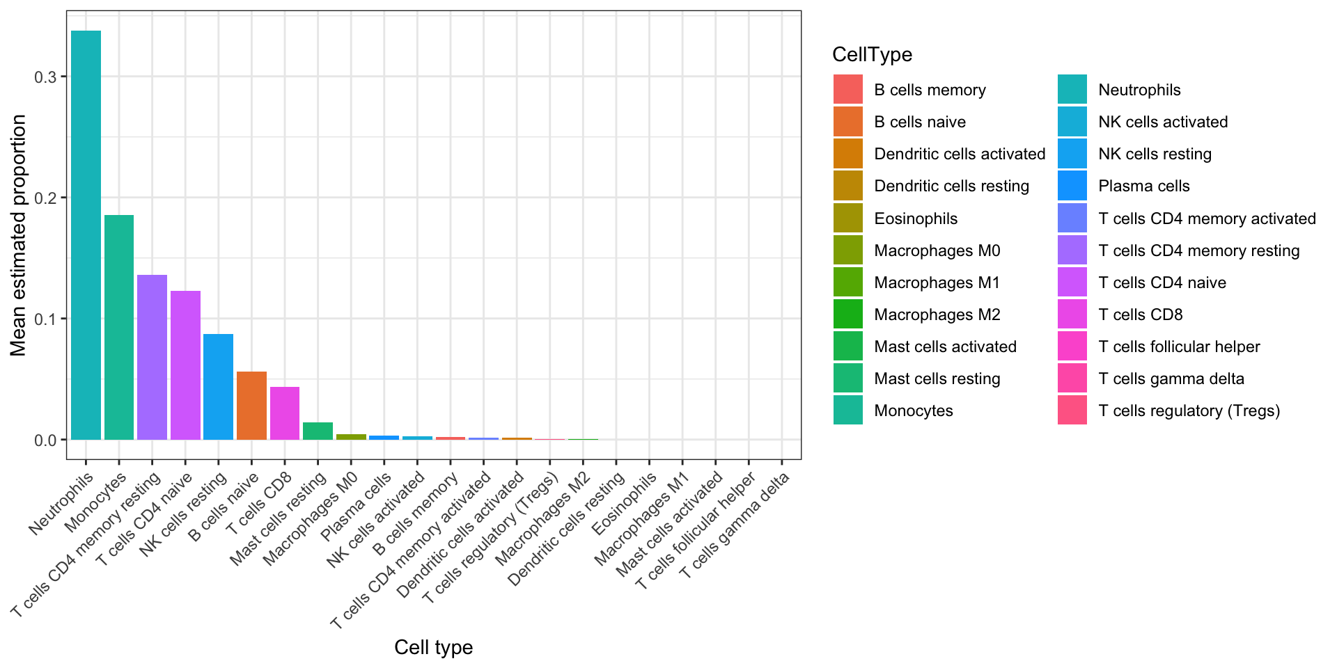

Past versions of "plot proportions-1.png"

Version	Author	Date
8802e57	sdhutchins	2026-04-14

Significant genes and heatmap

Keep gene–cell type pairs with q < 0.05, then within each cell type take the top 50 genes by GEP expression so the heatmap highlights strong, statistically supported signals, not every row of the matrix.

sig_genes <- qvals %>%
  rownames_to_column("Gene") %>%
  pivot_longer(-Gene, names_to = "CellType", values_to = "qval") %>%
  filter(qval < 0.05) %>%
  left_join(
    geps %>%
      rownames_to_column("Gene") %>%
      pivot_longer(-Gene, names_to = "CellType", values_to = "Expr"),
    by = c("Gene", "CellType")
  )

top_genes <- sig_genes %>%
  group_by(CellType) %>%
  top_n(50, Expr) %>%
  distinct(Gene, CellType, .keep_all = TRUE)

Row scaling (scale = "row") means each gene is centered to compare relative highs and lows across cell types, not absolute TPM-like units.

gene_subset <- intersect(rownames(geps), unique(top_genes$Gene))

if (length(gene_subset) == 0) {
  warning("No matching genes for heatmap; check gene IDs.")
} else {
  mat <- geps[rownames(geps) %in% gene_subset, ]
  mat[!is.finite(mat)] <- 0
  pheatmap(
    mat,
    scale = "row",
    clustering_distance_cols = "correlation",
    show_rownames = FALSE,
    main = "Top expressed genes across cell types"
  )
}

GO enrichment

enrichGO(..., ont = "BP") tests whether the gene list for each cell type overlaps known biological process terms more than chance; adjusted p-values rank pathways.

enrichment_results <- list()

for (ct in unique(top_genes$CellType)) {
  genes_ct <- top_genes %>% filter(CellType == ct) %>% pull(Gene)
  if (length(genes_ct) == 0) next

  ego <- enrichGO(
    gene = genes_ct,
    OrgDb = org.Hs.eg.db,
    keyType = "SYMBOL",
    ont = "BP",
    pAdjustMethod = "BH",
    qvalueCutoff = 0.05
  )
  enrichment_results[[ct]] <- ego
  print(head(ego@result[, c("Description", "p.adjust")], 5))
}

The dotplot is one representative cell type (first non-empty enrichment object); open the printed tables above for others.

if (length(enrichment_results) > 0) {
  dotplot(enrichment_results[[1]], showCategory = 10)
}

Save outputs (Job 1)

Write CSV summaries so Job 1 results are usable outside this R session (output/deconvolution/).

write_csv(fractions_summary, file.path(out_dir, "Job1_CellTypeProportionSummary.csv"))
write_csv(top_genes, file.path(out_dir, "Job1_TopGenes_PerCellType.csv"))

CIBERSORTx Job 2: LM22 whole blood

Job 2 chunks mirror the standalone LM22 script. They load fractions, merge IDs and metadata, then run category and affected-status comparisons and plots.

library(tidyverse)
library(MASS)
library(FSA)
library(ggpubr)
library(RColorBrewer)
library(pheatmap)

CGDSID is the CIBERSORTx sample key; id_map.csv maps it to SampleID in the study metadata. df is the analysis-ready table: LM22 proportions plus all metadata columns.

out_dir_job2 <- file.path(out_dir, "job2")
dir.create(out_dir_job2, recursive = TRUE, showWarnings = FALSE)

fractions <- read_csv("data/CIBERSORTx_Job2_output/CIBERSORTx_Job2_Results.csv", show_col_types = FALSE)
colnames(fractions)[1] <- "CGDSID"
celltype_cols <- setdiff(colnames(fractions), c("CGDSID", "P-value", "Correlation", "RMSE"))
fractions <- fractions %>% mutate(across(all_of(celltype_cols), as.numeric))

id_map <- read_csv("data/id_map.csv", show_col_types = FALSE) %>%
  dplyr::select(PaperID, CGDSID) %>%
  dplyr::filter(!is.na(PaperID) & !is.na(CGDSID)) %>%
  dplyr::rename(SampleID = PaperID)

fractions <- fractions %>%
  left_join(id_map, by = "CGDSID") %>%
  relocate(SampleID, .before = CGDSID)

if (any(is.na(fractions$SampleID))) {
  warning("Some CGDSIDs were not found in id_map.csv")
  print(fractions %>% dplyr::filter(is.na(SampleID)) %>% dplyr::select(CGDSID))
}

meta <- read_csv("data/Metadata_2024_11_20.csv", show_col_types = FALSE)
df <- fractions %>% left_join(meta, by = c("SampleID" = "ID"))

write_csv(df, file.path(out_dir_job2, "Job2_CellTypeProportions_Merged.csv"))

Category-based contrasts

Category is the metadata grouping variable for this block (change group_var if you need another column). Tables and tests describe whether LM22 proportions differ across Category levels.

group_var <- "Category"

if (!group_var %in% names(df)) stop(paste("Grouping variable", group_var, "not found in metadata."))
if (any(is.na(df[[group_var]]))) warning("Some samples missing group information.")

summary_stats_category <- df %>%
  pivot_longer(all_of(celltype_cols), names_to = "CellType", values_to = "Proportion") %>%
  group_by(CellType, .data[[group_var]]) %>%
  summarise(
    mean = mean(Proportion, na.rm = TRUE),
    sd = sd(Proportion, na.rm = TRUE),
    n = sum(!is.na(Proportion)),
    .groups = "drop"
  )

summary_stats_category

# A tibble: 132 × 5
   CellType       Category       mean        sd     n
   <chr>          <chr>         <dbl>     <dbl> <int>
 1 B cells memory ENE        0.000961  0.00193      6
 2 B cells memory IMM        0.00131   0.00262      4
 3 B cells memory RBC        0.00525   0.0125       6
 4 B cells memory SOL        0.00288   0.00644      5
 5 B cells memory STR        0        NA            1
 6 B cells memory Unaffected 0.000532  0.000807     7
 7 B cells naive  ENE        0.0663    0.0286       6
 8 B cells naive  IMM        0.0447    0.0162       4
 9 B cells naive  RBC        0.0733    0.0446       6
10 B cells naive  SOL        0.0525    0.0302       5
# ℹ 122 more rows

write_csv(summary_stats_category, file.path(out_dir_job2, paste0("Job2_CellTypeSummary_By_", group_var, ".csv")))

This chunk performs per-cell-type non-parametric tests by Category, applies BH correction, and writes omnibus and Dunn post hoc outputs.

message(paste("Running non-parametric tests for", group_var, "..."))

df_test_category <- df %>% filter(!is.na(.data[[group_var]]))
test_results_category <- tibble(CellType = character(), p = numeric(), test = character())

for (ct in celltype_cols) {
  tmp <- df_test_category %>%
    dplyr::select(all_of(group_var), all_of(ct)) %>%
    dplyr::filter(!is.na(.data[[group_var]]), !is.na(.data[[ct]]))

  n_groups <- length(unique(tmp[[group_var]]))

  if (n_groups == 2 && all(table(tmp[[group_var]]) > 1)) {
    pval <- tryCatch(
      stats::wilcox.test(tmp[[ct]] ~ tmp[[group_var]])$p.value,
      error = function(e) NA_real_
    )
    test_results_category <- bind_rows(
      test_results_category,
      tibble(CellType = ct, p = pval, test = "Mann-Whitney U")
    )

  } else if (n_groups > 2 && all(table(tmp[[group_var]]) > 1)) {
    pval_kw <- tryCatch(
      stats::kruskal.test(tmp[[ct]] ~ tmp[[group_var]])$p.value,
      error = function(e) NA_real_
    )

    dunn_res <- tryCatch(
      FSA::dunnTest(tmp[[ct]] ~ tmp[[group_var]], method = "bh")$res,
      error = function(e) NULL
    )

    if (!is.null(dunn_res)) {
      dunn_res <- dunn_res %>%
        mutate(
          CellType = ct,
          test = "Kruskal-Wallis + Dunn",
          comparison = Contrast
        ) %>%
        rename(p = P.unadj, p.adj = P.adj)
      write_csv(dunn_res, file.path(out_dir_job2, paste0("Job2_DunnResults_", ct, "_By_", group_var, ".csv")))
    }

    test_results_category <- bind_rows(
      test_results_category,
      tibble(CellType = ct, p = pval_kw, test = "Kruskal-Wallis")
    )
  }
}

test_results_category <- test_results_category %>%
  mutate(
    p.adj = p.adjust(p, method = "BH"),
    significance = case_when(
      is.na(p.adj) ~ "",
      p.adj < 0.001 ~ "***",
      p.adj < 0.01 ~ "**",
      p.adj < 0.05 ~ "*",
      TRUE ~ "ns"
    )
  )

test_results_category

# A tibble: 0 × 5
# ℹ 5 variables: CellType <chr>, p <dbl>, test <chr>, p.adj <dbl>,
#   significance <chr>

write_csv(test_results_category, file.path(out_dir_job2, paste0("Job2_GroupComparisonResults_By_", group_var, ".csv")))

We fit the Category-based ordered logistic model on quartiled neutrophil proportions and print both coefficients and odds ratios.

df_quart <- df_test_category %>%
  mutate(across(all_of(celltype_cols), ~ ntile(., 4), .names = "{.col}_quart"))

if (length(unique(df_quart$Category)) >= 2 && length(unique(df_quart$Sex)) >= 2) {
  model <- polr(as.factor(Neutrophils_quart) ~ Category + Sex, data = df_quart, Hess = TRUE)

  print(summary(model))
  print(exp(coef(model)))
}

Call:
polr(formula = as.factor(Neutrophils_quart) ~ Category + Sex, 
    data = df_quart, Hess = TRUE)

Coefficients:
                      Value Std. Error   t value
CategoryIMM         1.46130  1.337e+00 1.093e+00
CategoryRBC         0.08858  1.083e+00 8.178e-02
CategorySOL         1.30304  1.087e+00 1.198e+00
CategorySTR        17.44210  7.117e-07 2.451e+07
CategoryUnaffected  0.25565  1.091e+00 2.343e-01
SexM                1.50347  1.207e+00 1.246e+00

Intercepts:
    Value         Std. Error    t value      
1|2       -0.2948        0.8277       -0.3562
2|3        0.9113        0.8506        1.0714
3|4        2.1685        0.9337        2.3224

Residual Deviance: 73.65708 
AIC: 91.65708 
       CategoryIMM        CategoryRBC        CategorySOL        CategorySTR 
      4.311565e+00       1.092617e+00       3.680472e+00       3.758449e+07 
CategoryUnaffected               SexM 
      1.291294e+00       4.497272e+00 

This panel plot shows cell-type-specific proportion differences by Category with significance annotations from the test results.

plot_df <- df_test_category %>%
  pivot_longer(all_of(celltype_cols), names_to = "CellType", values_to = "Proportion")

sig_df <- test_results_category %>%
  dplyr::mutate(
    group1 = levels(factor(df_test_category$Category))[1],
    group2 = levels(factor(df_test_category$Category))[2],
    y.position = 1.05 * max(plot_df$Proportion, na.rm = TRUE)
  ) %>%
  dplyr::select(CellType, group1, group2, p.adj, significance, y.position) %>%
  dplyr::rename(p = p.adj)

p <- ggpubr::ggboxplot(
  plot_df,
  x = "Category",
  y = "Proportion",
  fill = "Category",
  outlier.shape = NA
) +
  facet_wrap(~ CellType, scales = "free_y", ncol = 4) +
  ggpubr::stat_pvalue_manual(
    sig_df,
    label = "significance",
    tip.length = 0.01,
    bracket.size = 0.3,
    hide.ns = TRUE
  ) +
  labs(
    title = "CIBERSORTx LM22 Immune Cell Proportions by Category",
    subtitle = "Boxplots with Mann-Whitney / Kruskal-Wallis significance annotations",
    y = "Estimated Proportion",
    x = NULL
  ) +
  theme_bw() +
  theme(
    strip.text = element_text(size = 9, face = "bold"),
    axis.text.x = element_text(angle = 45, hjust = 1),
    legend.position = "bottom"
  )

p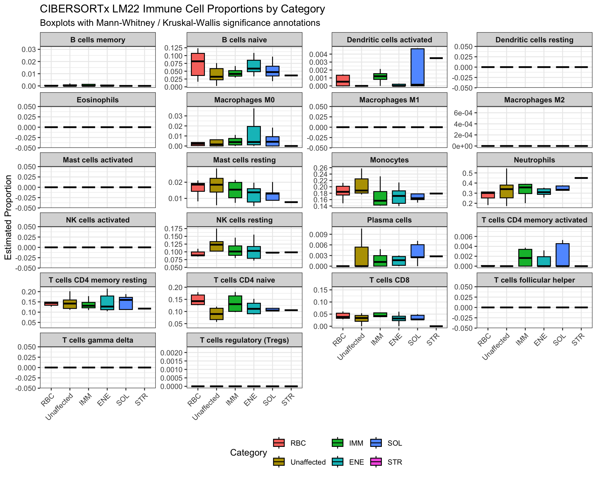

Past versions of "job2 category boxplots-1.png"

Version	Author	Date
8802e57	sdhutchins	2026-04-14

ggsave(file.path(out_dir_job2, "Job2_CellType_Boxplots_byCategory.png"), p, width = 10, height = 8, dpi = 300)

Affected-status contrasts

These tables use the same LM22 proportions as above, grouped by Affected instead of Category. Each table row gives mean, SD, and n for a cell type within Affected or Unaffected.

if (any(is.na(df$Affected))) warning("Some samples missing group information.")

summary_stats_affected <- df %>%
  pivot_longer(all_of(celltype_cols), names_to = "CellType", values_to = "Proportion") %>%
  group_by(CellType, Affected) %>%
  summarise(
    mean = mean(Proportion, na.rm = TRUE),
    sd = sd(Proportion, na.rm = TRUE),
    n = sum(!is.na(Proportion)),
    .groups = "drop"
  )

summary_stats_affected

# A tibble: 44 × 5
   CellType                  Affected        mean       sd     n
   <chr>                     <chr>          <dbl>    <dbl> <int>
 1 B cells memory            Affected   0.00259   0.00711     22
 2 B cells memory            Unaffected 0.000532  0.000807     7
 3 B cells naive             Affected   0.0598    0.0320      22
 4 B cells naive             Unaffected 0.0390    0.0278       7
 5 Dendritic cells activated Affected   0.00105   0.00149     22
 6 Dendritic cells activated Unaffected 0.0000742 0.000196     7
 7 Dendritic cells resting   Affected   0         0           22
 8 Dendritic cells resting   Unaffected 0         0            7
 9 Eosinophils               Affected   0         0           22
10 Eosinophils               Unaffected 0         0            7
# ℹ 34 more rows

write_csv(summary_stats_affected, file.path(out_dir_job2, "Job2_CellTypeSummary_ByGroup.csv"))

This chunk runs Mann-Whitney comparisons for each cell type between Affected and Unaffected groups and adds BH-adjusted significance labels.

message("Running non-parametric group comparisons (Mann-Whitney U)...")

df_test_affected <- df %>% dplyr::filter(!is.na(Affected))
test_results_affected <- tibble::tibble(CellType = character(), p = numeric())

for (ct in celltype_cols) {
  tmp <- df_test_affected %>%
    dplyr::select(Affected, !!sym(ct)) %>%
    dplyr::filter(!is.na(Affected), !is.na(!!sym(ct)))

  if (length(unique(tmp$Affected)) == 2 &&
      all(table(tmp$Affected) > 1)) {

    pval <- tryCatch({
      stats::wilcox.test(tmp[[ct]] ~ tmp$Affected)$p.value
    }, error = function(e) NA_real_)

    test_results_affected <- dplyr::bind_rows(
      test_results_affected,
      tibble::tibble(CellType = ct, p = pval)
    )
  }
}

test_results_affected <- test_results_affected %>%
  dplyr::mutate(
    p.adj = p.adjust(p, method = "BH"),
    significance = dplyr::case_when(
      is.na(p.adj) ~ "",
      p.adj < 0.001 ~ "***",
      p.adj < 0.01 ~ "**",
      p.adj < 0.05 ~ "*",
      TRUE ~ "ns"
    )
  )

test_results_affected

# A tibble: 22 × 4
   CellType                           p   p.adj significance
   <chr>                          <dbl>   <dbl> <chr>       
 1 B cells naive                  0.149   0.543 "ns"        
 2 B cells memory                 0.686   0.878 "ns"        
 3 Plasma cells                   0.978   1     "ns"        
 4 T cells CD8                    0.702   0.878 "ns"        
 5 T cells CD4 naive              0.181   0.543 "ns"        
 6 T cells CD4 memory resting     0.901   1     "ns"        
 7 T cells CD4 memory activated   0.226   0.564 "ns"        
 8 T cells follicular helper    NaN     NaN     ""          
 9 T cells regulatory (Tregs)     0.451   0.846 "ns"        
10 T cells gamma delta          NaN     NaN     ""          
# ℹ 12 more rows

readr::write_csv(test_results_affected, file.path(out_dir_job2, "Job2_GroupComparisonResults.csv"))

We fit the ordered logistic model using quartiled neutrophil proportions against Affected status and Sex.

df_quart <- df_test_affected %>%
  mutate(across(all_of(celltype_cols), ~ ntile(., 4), .names = "{.col}_quart"))

model <- polr(as.factor(Neutrophils_quart) ~ Affected + Sex, data = df_quart, Hess = TRUE)
summary(model)

Call:
polr(formula = as.factor(Neutrophils_quart) ~ Affected + Sex, 
    data = df_quart, Hess = TRUE)

Coefficients:
                     Value Std. Error t value
AffectedUnaffected -0.3962     0.9014 -0.4395
SexM                1.0904     1.1761  0.9271

Intercepts:
    Value   Std. Error t value
1|2 -0.9412  0.4535    -2.0755
2|3  0.1215  0.4141     0.2934
3|4  1.2015  0.4821     2.4921

Residual Deviance: 79.38353 
AIC: 89.38353 

exp(coef(model))

AffectedUnaffected               SexM 
         0.6729055          2.9753320 

This faceted boxplot visualizes Affected-group differences per cell type with significance stars from the tested contrasts.

plot_df <- df_test_affected %>%
  tidyr::pivot_longer(all_of(celltype_cols), names_to = "CellType", values_to = "Proportion")

sig_df <- test_results_affected %>%
  dplyr::mutate(
    group1 = "Unaffected",
    group2 = "Affected",
    y.position = 1.05 * max(plot_df$Proportion, na.rm = TRUE)
  ) %>%
  dplyr::select(CellType, group1, group2, p.adj, significance, y.position) %>%
  dplyr::rename(p = p.adj)

p <- ggpubr::ggboxplot(
  plot_df,
  x = "Affected",
  y = "Proportion",
  fill = "Affected",
  palette = c("#4575b4", "#d73027"),
  outlier.shape = NA
) +
  facet_wrap(~ CellType, scales = "free_y", ncol = 4) +
  ggpubr::stat_pvalue_manual(
    sig_df,
    label = "significance",
    tip.length = 0.01,
    bracket.size = 0.3,
    hide.ns = TRUE
  ) +
  labs(
    title = "CIBERSORTx LM22 Immune Cell Proportions by Affected Status",
    subtitle = "Boxplots with Mann-Whitney significance annotations",
    y = "Estimated Proportion",
    x = NULL
  ) +
  theme_bw() +
  theme(
    strip.text = element_text(size = 9, face = "bold"),
    axis.text.x = element_text(angle = 45, hjust = 1),
    legend.position = "bottom"
  )

print(p)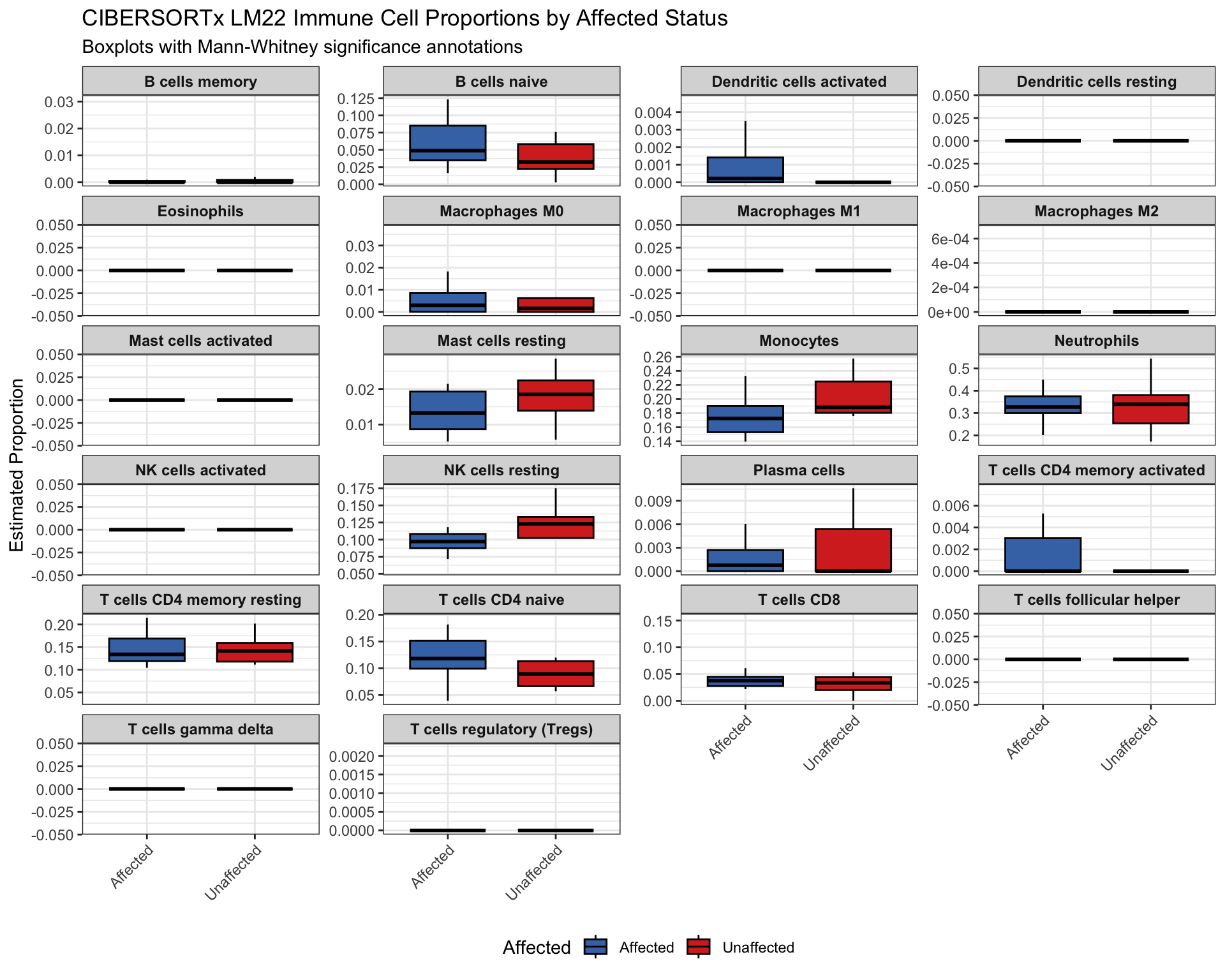

Past versions of "job2 affected boxplots-1.png"

Version	Author	Date
8802e57	sdhutchins	2026-04-14

ggplot2::ggsave(file.path(out_dir_job2, "Job2_CellType_Boxplots_with_Significance.png"), p, width = 10, height = 8, dpi = 300)

Sample-level composition plots

In the stacked bar charts, each bar sums to height 1 per sample, and each segment height is that sample’s LM22 fraction for a cell type. Samples are ordered within Affected so you can scan homogeneous runs of composition.

palette22 <- colorRampPalette(brewer.pal(12, "Set3"))(22)

plot_df <- df %>%
  pivot_longer(all_of(celltype_cols), names_to = "CellType", values_to = "Proportion") %>%
  group_by(SampleID, Affected, CellType) %>%
  summarise(Proportion = mean(Proportion, na.rm = TRUE), .groups = "drop")

plot_df <- plot_df %>%
  arrange(Affected, SampleID) %>%
  mutate(SampleID = factor(SampleID, levels = unique(SampleID)))

g_affected <- ggplot(plot_df, aes(x = SampleID, y = Proportion, fill = CellType)) +
  geom_bar(stat = "identity", width = 0.8, color = "white", size = 0.1) +
  scale_fill_manual(values = palette22) +
  labs(
    title = "CIBERSORTx LM22 Immune Composition per Sample",
    subtitle = "Samples grouped by clinical status (Affected vs Unaffected)",
    y = "Relative proportion",
    x = "Sample ID",
    fill = "Cell type"
  ) +
  theme_bw(base_size = 11) +
  theme(
    axis.text.x = element_text(angle = 90, vjust = 0.5, hjust = 1, size = 7, color = "grey20"),
    axis.title.y = element_text(size = 10),
    panel.grid.major.x = element_blank(),
    panel.grid.minor.x = element_blank(),
    strip.text = element_text(face = "bold", size = 10),
    legend.position = "right",
    legend.title = element_text(face = "bold", size = 9),
    legend.text = element_text(size = 8)
  ) +
  geom_vline(
    xintercept = length(unique(plot_df$SampleID[plot_df$Affected == "Unaffected"])) + 0.5,
    color = "black",
    linewidth = 0.6,
    linetype = "dashed"
  ) +
  annotate(
    "text",
    x = length(unique(plot_df$SampleID[plot_df$Affected == "Unaffected"])) / 2,
    y = 1.05,
    label = "Unaffected",
    fontface = "bold",
    size = 3.5
  ) +
  annotate(
    "text",
    x = length(unique(plot_df$SampleID[plot_df$Affected == "Unaffected"])) +
      length(unique(plot_df$SampleID[plot_df$Affected == "Affected"])) / 2,
    y = 1.05,
    label = "Affected",
    fontface = "bold",
    size = 3.5
  )

g_affected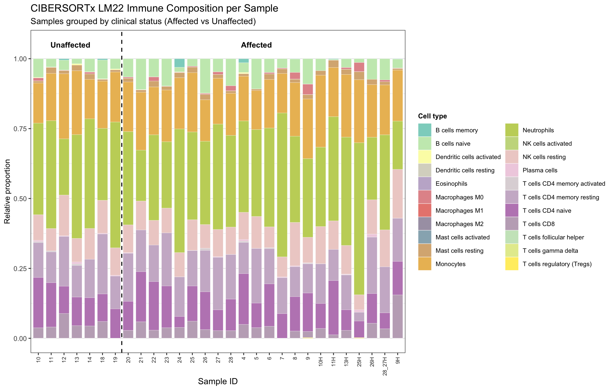

Past versions of "job2 affected stacked-bar-1.png"

Version	Author	Date
8802e57	sdhutchins	2026-04-14

ggsave(file.path(out_dir_job2, "Job2_StackedBar_By_Affected.png"), g_affected, width = 11, height = 7, dpi = 300)

This stacked bar chart repeats the same composition view but grouped and labeled by Category.

palette22 <- colorRampPalette(brewer.pal(12, "Set3"))(22)

plot_df <- df %>%
  pivot_longer(all_of(celltype_cols), names_to = "CellType", values_to = "Proportion") %>%
  group_by(SampleID, Category, CellType) %>%
  summarise(Proportion = mean(Proportion, na.rm = TRUE), .groups = "drop") %>%
  arrange(Category, SampleID) %>%
  mutate(SampleID = factor(SampleID, levels = unique(SampleID)))

g_category <- ggplot(plot_df, aes(x = SampleID, y = Proportion, fill = CellType)) +
  geom_bar(stat = "identity", width = 0.8, color = "white", size = 0.1) +
  scale_fill_manual(values = palette22) +
  labs(
    title = "CIBERSORTx LM22 Immune Composition per Sample",
    subtitle = "Samples grouped by Category",
    y = "Relative proportion",
    x = "Sample ID",
    fill = "Cell type"
  ) +
  theme_bw(base_size = 11) +
  theme(
    axis.text.x = element_text(angle = 90, vjust = 0.5, hjust = 1, size = 7, color = "grey20"),
    axis.title.y = element_text(size = 10),
    panel.grid.major.x = element_blank(),
    panel.grid.minor.x = element_blank(),
    legend.position = "right",
    legend.title = element_text(face = "bold", size = 9),
    legend.text = element_text(size = 8)
  ) +
  {
    cat_counts <- plot_df %>%
      distinct(SampleID, Category) %>%
      count(Category) %>%
      mutate(x_mid = cumsum(n) - n / 2, x_div = cumsum(n) + 0.5)

    list(
      geom_vline(
        data = cat_counts[-nrow(cat_counts), ],
        aes(xintercept = x_div),
        color = "black",
        linewidth = 0.6,
        linetype = "dashed"
      ),
      geom_text(
        data = cat_counts,
        aes(x = x_mid, y = 1.05, label = Category),
        fontface = "bold",
        size = 3.5,
        inherit.aes = FALSE
      )
    )
  }

g_category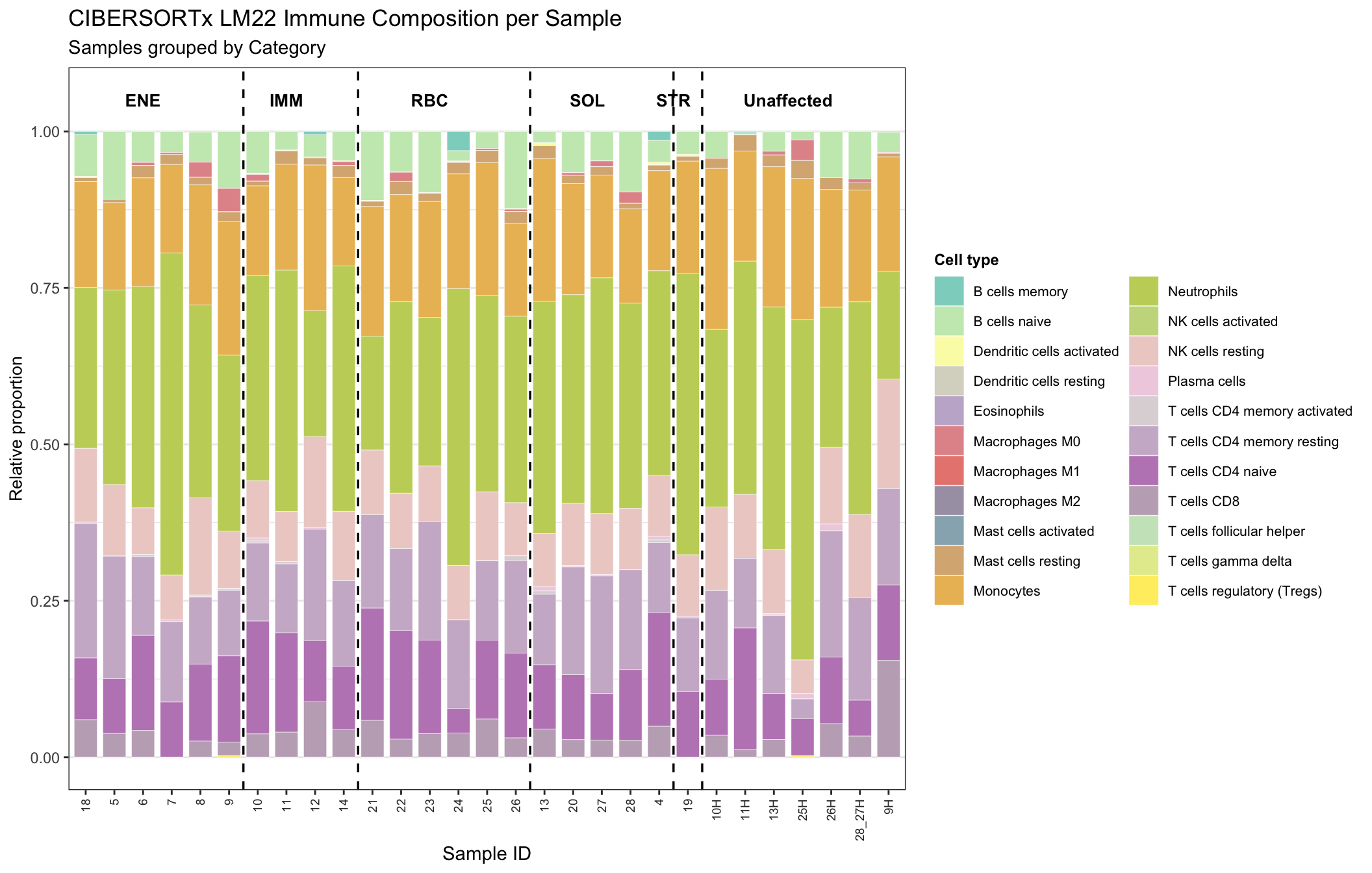

Past versions of "job2 category stacked-bar-1.png"

Version	Author	Date
8802e57	sdhutchins	2026-04-14

ggsave(file.path(out_dir_job2, "Job2_StackedBar_By_Category.png"), g_category, width = 11, height = 7, dpi = 300)

Multivariate summaries

PCA on fraction columns treats each sample as a vector of cell-type proportions; scale. = TRUE gives each cell type equal weight. Constant columns (zero variance) are dropped so prcomp() does not fail.

group_var <- "Category"

pca_data <- df %>% dplyr::select(all_of(celltype_cols)) %>% drop_na()
constant_cols <- names(which(apply(pca_data, 2, sd, na.rm = TRUE) == 0))

if (length(constant_cols) > 0) {
  message("Removing constant columns from PCA: ", paste(constant_cols, collapse = ", "))
  pca_data <- pca_data %>% dplyr::select(-all_of(constant_cols))
}

if (nrow(pca_data) > 2 && ncol(pca_data) > 1) {
  pca_res <- prcomp(pca_data, scale. = TRUE)

  pca_df <- as.data.frame(pca_res$x[, 1:2]) %>%
    mutate(
      SampleID = df$SampleID[complete.cases(pca_data)],
      Group = df[[group_var]][complete.cases(pca_data)]
    )

  pca_plot <- ggplot(pca_df, aes(PC1, PC2, color = Group, label = SampleID)) +
    geom_point(size = 3, alpha = 0.9) +
    ggrepel::geom_text_repel(size = 2.8, max.overlaps = 20, segment.color = "grey50") +
    theme_bw() +
    labs(
      title = paste("PCA of CIBERSORTx Immune Cell Proportions by", group_var),
      subtitle = "Each point represents one individual sample",
      x = paste0("PC1 (", round(summary(pca_res)$importance[2,1] * 100, 1), "% variance)"),
      y = paste0("PC2 (", round(summary(pca_res)$importance[2,2] * 100, 1), "% variance)")
    ) +
    theme(
      legend.position = "bottom",
      legend.title = element_text(face = "bold"),
      plot.title = element_text(face = "bold")
    )

  pca_plot
  ggsave(file.path(out_dir_job2, paste0("Job2_PCA_By_", group_var, "_Labeled.png")),
         pca_plot, width = 8, height = 6, dpi = 300)
} else {
  warning("Not enough variable cell types for PCA.")
}

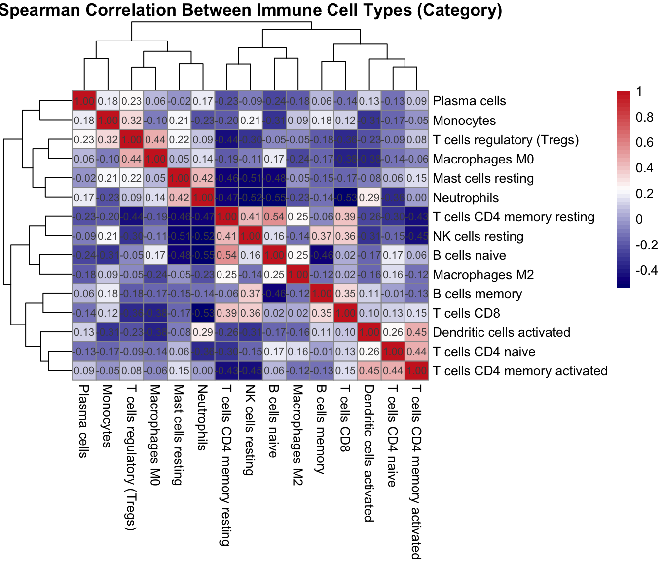
This chunk computes a Spearman correlation matrix across immune cell types and displays the clustered heatmap.

df_corr <- df %>%
  dplyr::select(all_of(celltype_cols)) %>%
  dplyr::select(where(is.numeric))

df_corr <- df_corr[, apply(df_corr, 2, function(x) var(x, na.rm = TRUE) > 0.0 & sum(!is.na(x)) > 2)]

corr_matrix <- suppressWarnings(cor(df_corr, method = "spearman", use = "pairwise.complete.obs"))
corr_matrix[is.na(corr_matrix)] <- 0

pheatmap(
  corr_matrix,
  color = colorRampPalette(c("navy", "white", "firebrick3"))(50),
  display_numbers = TRUE,
  number_format = "%.2f",
  fontsize_number = 8,
  cluster_rows = TRUE,
  cluster_cols = TRUE,
  main = paste("Spearman Correlation Between Immune Cell Types (", group_var, ")", sep = "")
)

Past versions of "job2 correlation heatmap-1.png"

Version	Author	Date
8802e57	sdhutchins	2026-04-14

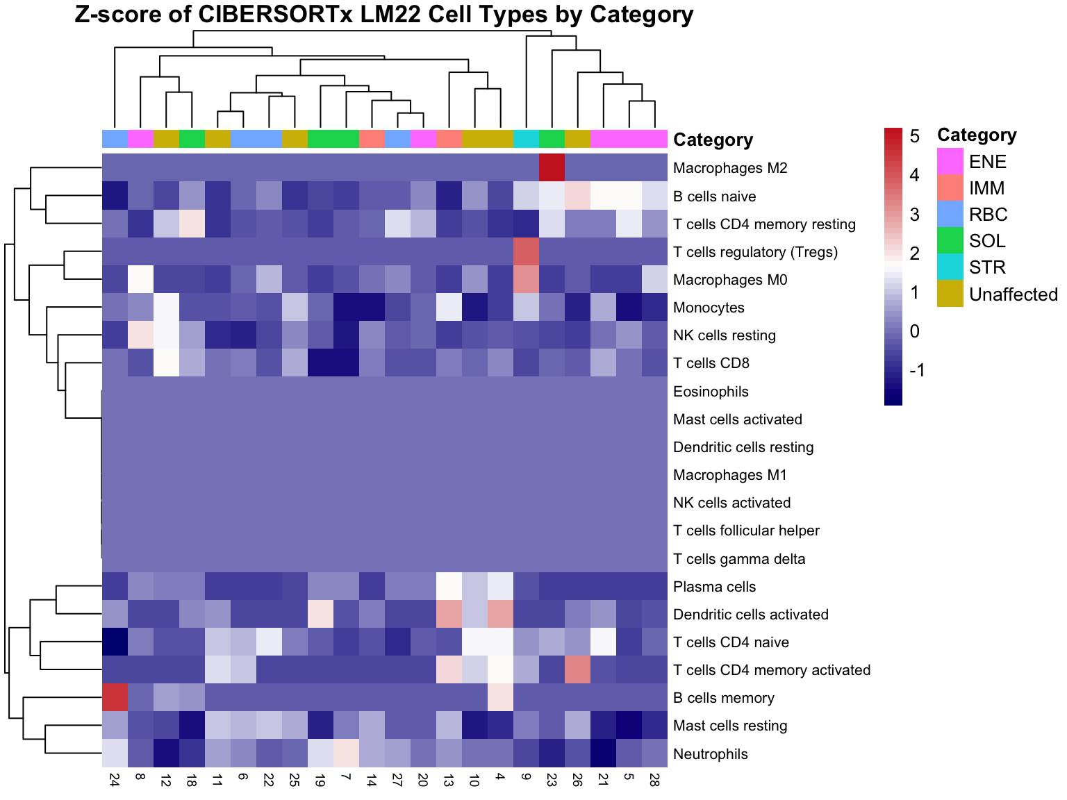
Here we z-score cell-type fractions across samples and plot a Category-annotated heatmap for relative composition patterns.

z_mat <- df %>%
  dplyr::select(SampleID, all_of(celltype_cols)) %>%
  tibble::column_to_rownames("SampleID") %>%
  as.matrix()

z_mat <- scale(z_mat)
stopifnot(is.numeric(z_mat))
z_mat[!is.finite(z_mat)] <- 0

annotation_df <- df %>%
  dplyr::select(SampleID, Category) %>%
  dplyr::filter(!is.na(Category)) %>%
  dplyr::distinct(SampleID, .keep_all = TRUE)
rownames(annotation_df) <- annotation_df$SampleID
annotation_df <- as.data.frame(annotation_df["Category"])
annotation_df$Category <- as.factor(annotation_df$Category)

common_samples <- intersect(rownames(z_mat), rownames(annotation_df))
z_mat <- z_mat[common_samples, , drop = FALSE]
annotation_df <- annotation_df[common_samples, , drop = FALSE]

pheatmap(
  t(z_mat),
  annotation_col = annotation_df,
  color = colorRampPalette(c("navy", "white", "firebrick3"))(50),
  cluster_cols = TRUE,
  cluster_rows = TRUE,
  show_colnames = TRUE,
  show_rownames = TRUE,
  fontsize_row = 8,
  fontsize_col = 7,
  border_color = NA,
  main = paste("Z-score of CIBERSORTx LM22 Cell Types by", group_var)
)

Past versions of "job2 zscore heatmap-1.png"

Version	Author	Date
8802e57	sdhutchins	2026-04-14

This final distribution plot shows overall predicted cell-frequency patterns per cell type using violin and embedded boxplots.

plot_df <- df %>%
  pivot_longer(all_of(celltype_cols), names_to = "CellType", values_to = "Proportion") %>%
  dplyr::filter(!is.na(Proportion))

median_order <- plot_df %>%
  group_by(CellType) %>%
  summarise(median_val = median(Proportion, na.rm = TRUE)) %>%
  arrange(desc(median_val)) %>%
  pull(CellType)

plot_df$CellType <- factor(plot_df$CellType, levels = median_order)

fill_color <- "#A6CEE3"
box_color <- "#1F78B4"

p <- ggplot(plot_df, aes(x = CellType, y = Proportion)) +
  geom_violin(fill = fill_color, color = "gray40", width = 0.9, scale = "width", alpha = 0.9) +
  geom_boxplot(width = 0.12, color = "black", fill = box_color, outlier.shape = NA, alpha = 0.7) +
  labs(
    title = "Predicted relative frequency of immune cell types in whole blood",
    x = "Immune cell type",
    y = "Predicted relative frequency"
  ) +
  theme_bw(base_size = 11) +
  theme(
    axis.text.x = element_text(angle = 45, hjust = 1, size = 9),
    axis.text.y = element_text(size = 9),
    panel.grid.major.x = element_blank(),
    panel.grid.minor = element_blank(),
    panel.border = element_blank(),
    plot.title = element_text(face = "bold", hjust = 0.5, size = 12),
    axis.title = element_text(size = 10)
  )

p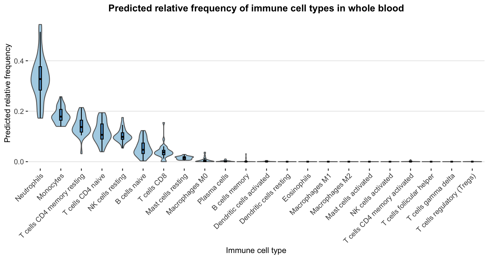

Past versions of "job2 violin boxplot-1.png"

Version	Author	Date
8802e57	sdhutchins	2026-04-14

ggsave(file.path(out_dir_job2, "Job2_ViolinBoxplot_CellFrequencies.png"), p, width = 8.5, height = 4.5, dpi = 300)

Session information

sessionInfo()

R version 4.5.1 (2025-06-13)
Platform: aarch64-apple-darwin20
Running under: macOS Tahoe 26.3

Matrix products: default
BLAS:   /Library/Frameworks/R.framework/Versions/4.5-arm64/Resources/lib/libRblas.0.dylib 
LAPACK: /Library/Frameworks/R.framework/Versions/4.5-arm64/Resources/lib/libRlapack.dylib;  LAPACK version 3.12.1

locale:
[1] en_US.UTF-8/en_US.UTF-8/en_US.UTF-8/C/en_US.UTF-8/en_US.UTF-8

time zone: America/Chicago
tzcode source: internal

attached base packages:
[1] stats4    stats     graphics  grDevices datasets  utils     methods  
[8] base     

other attached packages:
 [1] RColorBrewer_1.1-3     ggpubr_0.6.1           FSA_0.10.1            
 [4] MASS_7.3-65            org.Hs.eg.db_3.21.0    AnnotationDbi_1.70.0  
 [7] IRanges_2.42.0         S4Vectors_0.46.0       Biobase_2.68.0        
[10] BiocGenerics_0.54.0    generics_0.1.4         clusterProfiler_4.16.0
[13] pheatmap_1.0.13        lubridate_1.9.4        forcats_1.0.0         
[16] stringr_1.5.1          dplyr_1.1.4            purrr_1.1.0           
[19] readr_2.1.5            tidyr_1.3.1            tibble_3.3.0          
[22] ggplot2_3.5.2          tidyverse_2.0.0        workflowr_1.7.1       

loaded via a namespace (and not attached):
  [1] rstudioapi_0.17.1       jsonlite_2.0.0          magrittr_2.0.3         
  [4] ggtangle_0.0.7          farver_2.1.2            rmarkdown_2.29         
  [7] ragg_1.4.0              fs_1.6.6                vctrs_0.6.5            
 [10] memoise_2.0.1           ggtree_3.16.3           rstatix_0.7.2          
 [13] htmltools_0.5.8.1       broom_1.0.8             Formula_1.2-5          
 [16] gridGraphics_0.5-1      sass_0.4.10             bslib_0.9.0            
 [19] plyr_1.8.9              cachem_1.1.0            whisker_0.4.1          
 [22] igraph_2.1.4            lifecycle_1.0.4         pkgconfig_2.0.3        
 [25] Matrix_1.7-3            R6_2.6.1                fastmap_1.2.0          
 [28] gson_0.1.0              GenomeInfoDbData_1.2.14 digest_0.6.37          
 [31] aplot_0.2.8             enrichplot_1.28.4       colorspace_2.1-1       
 [34] patchwork_1.3.1         ps_1.9.1                rprojroot_2.1.0        
 [37] textshaping_1.0.1       RSQLite_2.4.2           labeling_0.4.3         
 [40] timechange_0.3.0        abind_1.4-8             httr_1.4.7             
 [43] compiler_4.5.1          bit64_4.6.0-1           withr_3.0.2            
 [46] backports_1.5.0         BiocParallel_1.42.1     carData_3.0-5          
 [49] DBI_1.2.3               R.utils_2.13.0          ggsignif_0.6.4         
 [52] tools_4.5.1             ape_5.8-1               httpuv_1.6.16          
 [55] R.oo_1.27.1             glue_1.8.0              callr_3.7.6            
 [58] nlme_3.1-168            GOSemSim_2.34.0         promises_1.3.3         
 [61] grid_4.5.1              getPass_0.2-4           reshape2_1.4.4         
 [64] fgsea_1.34.2            gtable_0.3.6            tzdb_0.5.0             
 [67] R.methodsS3_1.8.2       data.table_1.17.8       hms_1.1.3              
 [70] car_3.1-3               utf8_1.2.6              XVector_0.48.0         
 [73] ggrepel_0.9.6           pillar_1.11.0           yulab.utils_0.2.0      
 [76] vroom_1.6.5             later_1.4.2             splines_4.5.1          
 [79] treeio_1.32.0           lattice_0.22-7          renv_1.1.4             
 [82] bit_4.6.0               tidyselect_1.2.1        GO.db_3.21.0           
 [85] Biostrings_2.76.0       knitr_1.50              git2r_0.36.2           
 [88] xfun_0.52               stringi_1.8.7           UCSC.utils_1.4.0       
 [91] lazyeval_0.2.2          ggfun_0.2.0             yaml_2.3.10            
 [94] evaluate_1.0.4          codetools_0.2-20        qvalue_2.40.0          
 [97] BiocManager_1.30.26     ggplotify_0.1.2         cli_3.6.5              
[100] systemfonts_1.2.3       processx_3.8.6          jquerylib_0.1.4        
[103] Rcpp_1.1.0              GenomeInfoDb_1.44.0     png_0.1-8              
[106] parallel_4.5.1          blob_1.2.4              DOSE_4.2.0             
[109] tidytree_0.4.6          scales_1.4.0            crayon_1.5.3           
[112] rlang_1.1.6             cowplot_1.2.0           fastmatch_1.1-6        
[115] KEGGREST_1.48.1